Mathematics applied to well control

Basically the calculations used in the control of the well by the methods of the perforator and the engineer, especially the method of the engineer is due to the need to circulate the well to remove the influence of the well, it is also necessary to maintain the pressure at the bottom constant once the total volume of pumping reached the final pressure of circulation.

To achieve these well control objectives, there are applied well control mathematics that are used to calculate the density of a new control fluid.

Generally the math that is most often used is when the driller's method is applied, since the mathematical calculations involved are mostly applied to know exactly the density of the new control fluid.

Step-by-step description of the mathematical calculations required for well control

The first thing to do is to make the interpretation of the pressures, among these pressures are the formation pressure, which we can calculate if we have the reading of the closing pressures, among the closing pressures the one we are going to use for this case is the drill pipe closing pressure.

Once we close the well and wait for the closing pressures to stabilize, both in the drill pipe (SIDPP) and in the casing (SICP), we can calculate the formation pressure (Pform).

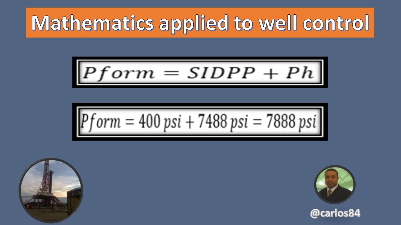
We proceed to calculate the formation pressure as follows:

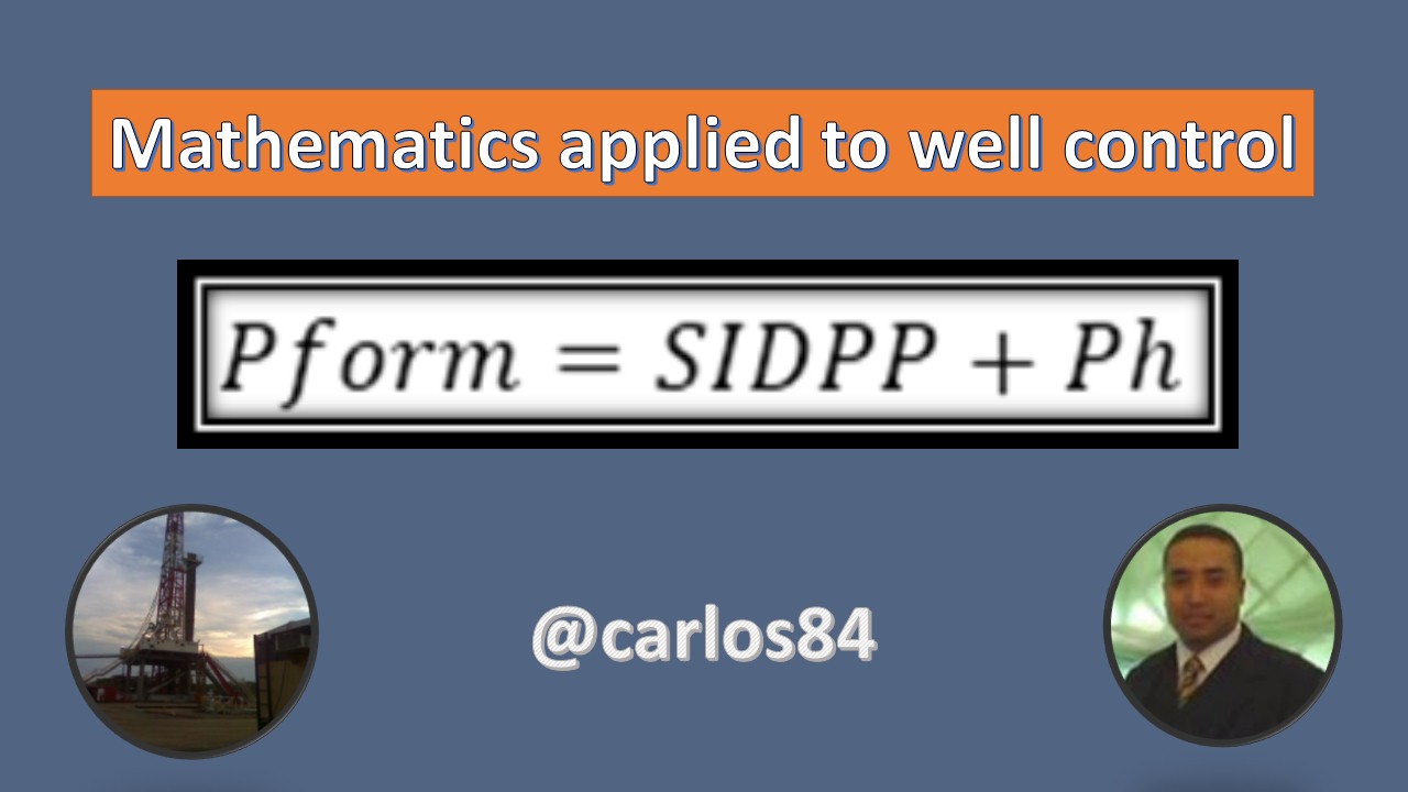
Pform: is the formation pressure at which the influx entered the well, measured in psi.

SIDPP: is the closing pressure of the stabilized drill pipe, and represents the difference in favour of the formation pressure with respect to the Ph (hydrostatic pressure of the drilling fluid). This pressure is measured in psi.

Ph: hydrostatic pressure of the drilling fluid, measured in psi, and is calculated as follows:

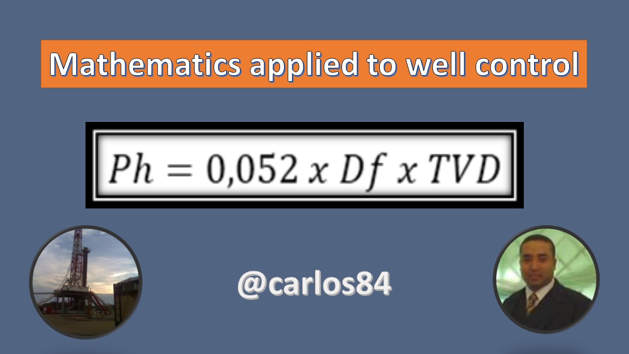
Df: is the density of the drilling fluid (mud), measured in pounds/gallon.

TVD: is the true vertical depth, measured in feet.

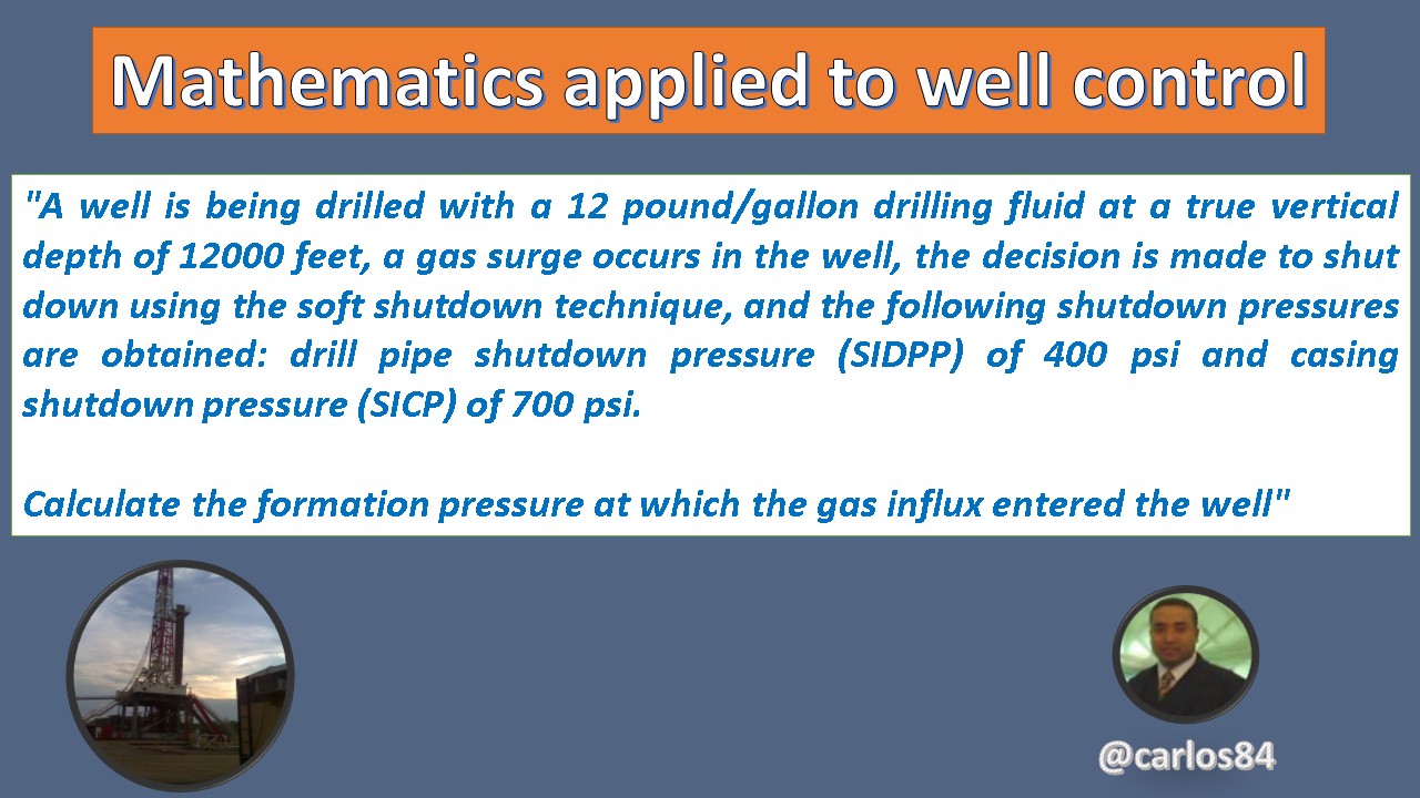
Exercise where the closure of a well is applied, and we want to find the formation pressure with which the fluids enter the well:

Solution

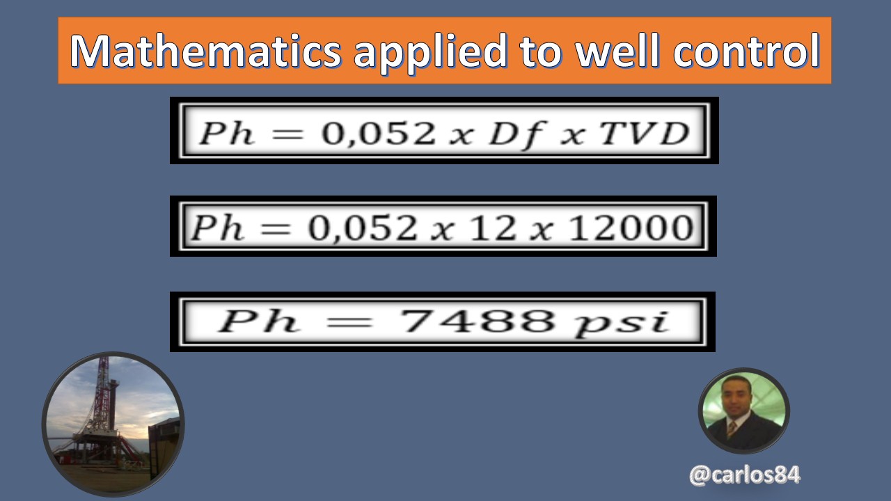
The first thing we have to calculate is the hydrostatic pressure.

As a second step we have to substitute the drill pipe closing pressure and the value we calculated of hydrostatic pressure in the equation for the formation pressure calculation:

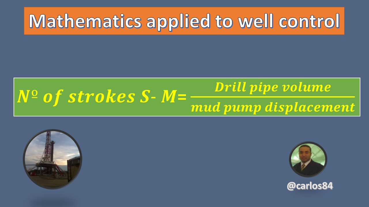
We calculate the number of strokes of the slurry pump from the surface to the wick (No. of strokes S-M).

If we take into account that the pipe volume and the displacement of the pump, are data that we must have tabulated in the drill, then we can calculate the number of strokes from the surface to the wick as follows:

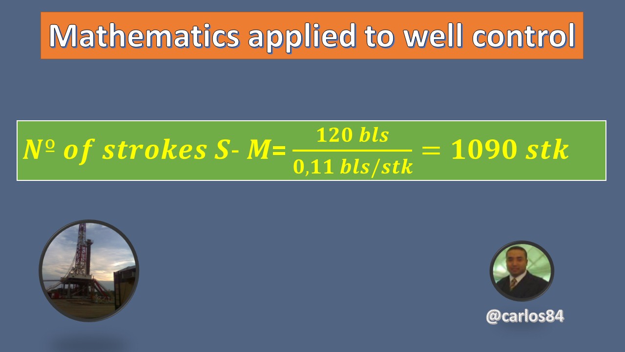
For example, suppose we have a pipe string whose volume is 120 barrels, and we have a triplex pump whose displacement is 0.11 barrels/stroke, we can calculate the number of strokes from the surface to the wick as follows:

We calculate the time from the surface to the wick (S-M time):

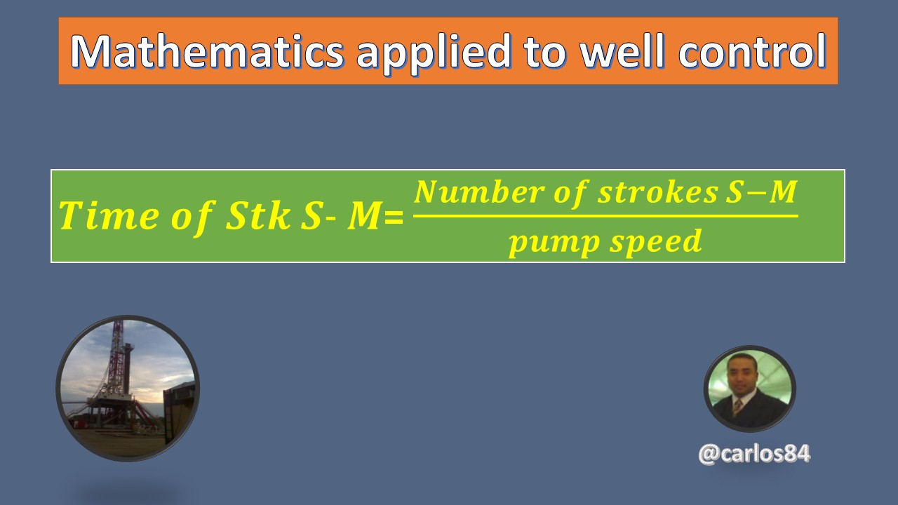
The speed of the pump is the one selected to perform the well control, that is the speed to circulate the well, this speed is measured in strokes per minute (SPM). Generally, a speed of 40 SPM is used for well control.

For example, calculate the time to pump the 1090 strokes from the surface to the wick, taking into account that a pump speed of 40 strokes per minute (SPM) is used.

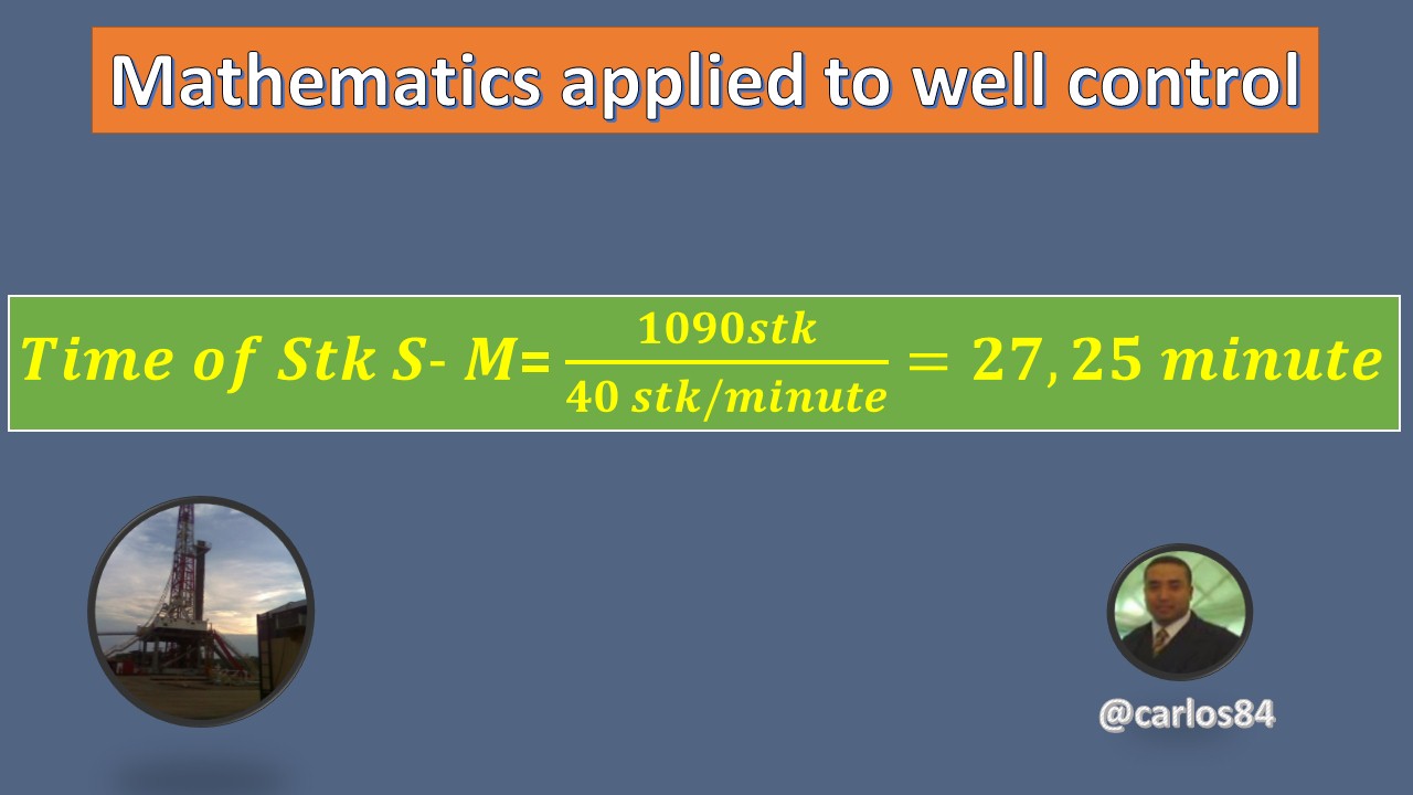
It will take 27.25 minutes to pump 1090 wrapped from the surface to the wick.

Number of strokes from the wick to the surface (No. of M-S strokes).It is important to mention that the annular volume is the volume occupied by the drilling fluid in the existing annular space. This annular space is between:

Drill pipe and hole.

Drill pipe and casing. These casings vary in diameter, so that an annular volume must be calculated for the different diameters.

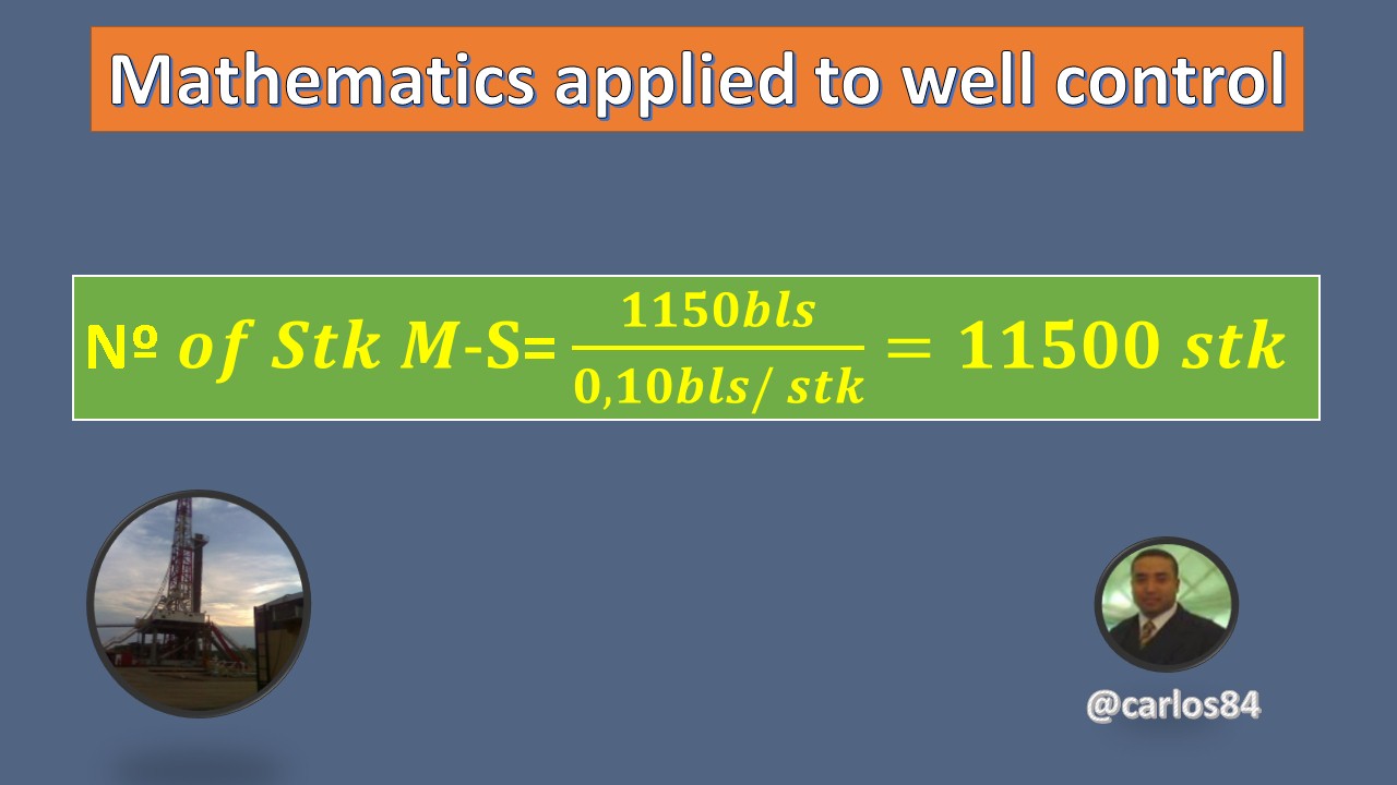
This annular volume should have been calculated in the borehole prior to well control. These calculations will depend on the diameters of the pipes that make up the drill string, i.e. drill collars and heavy weight pipes have a different diameter than drill pipes. Below is an example of how to calculate the number of strokes from the drill string to the surface:

You have an annular space in a well whose volume is 1150 barrels, you also have a triplex mud pump with a displacement of 0.10 barrels for each stroke. Calculate the number of strokes from the wick to the surface.

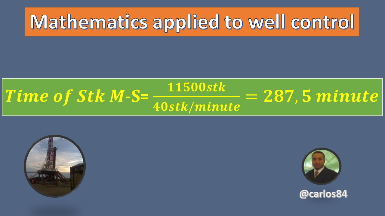
Time from Wick to Surface (M-S Time).

Initial circulation pressure (PIC)

This is the pressure with which we are going to start pumping mud to circulate the emergence and is nothing more than the sum of the drill pipe pressure and the reduced pumping pressure.

Control density (KMW)

It is the density of the new fluid with which we are going to control the well, it is worth mentioning that this density is higher than the original fluid.

Final circulation pressure (PFC)

The final circulation pressure is the pressure at which we will finish pumping the sludge.

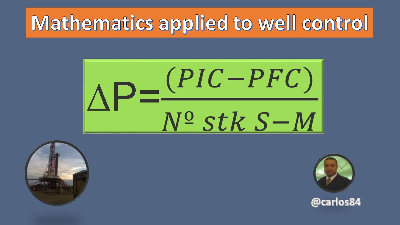
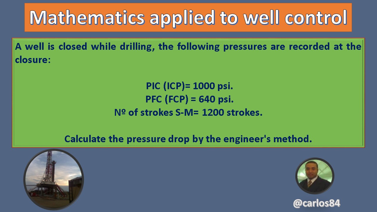
Calculate the pressure drop by the engineer's method (∆P)

This pressure differential tells us that, as we increase the pump strokes, the circulation pressure falls until it reaches the final circulation pressure, the question is at what rate this pressure must fall for the unwanted influence to enter again, for this we calculate this pressure drop as follows:

Apply a well control exercise by the engineer's method

To calculate the pressure drop by the engineer's method we simply subtract the final circulation pressure from the initial circulation pressure, this pressure differential will be divided by the 1200 strokes of the pump.

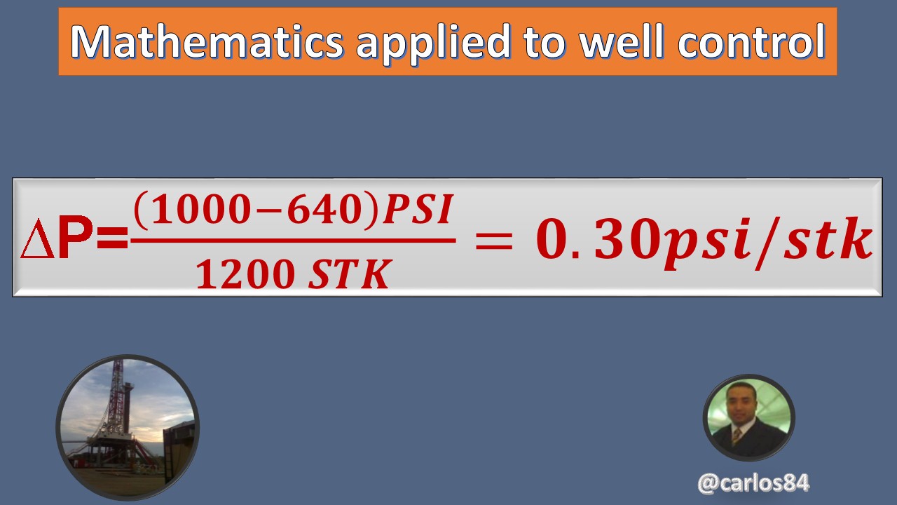
The result of a drop of 0.30 psi for each stroke made by the mud pump which means that for each stroke of the pump you will have a pressure of 0.30 psi.

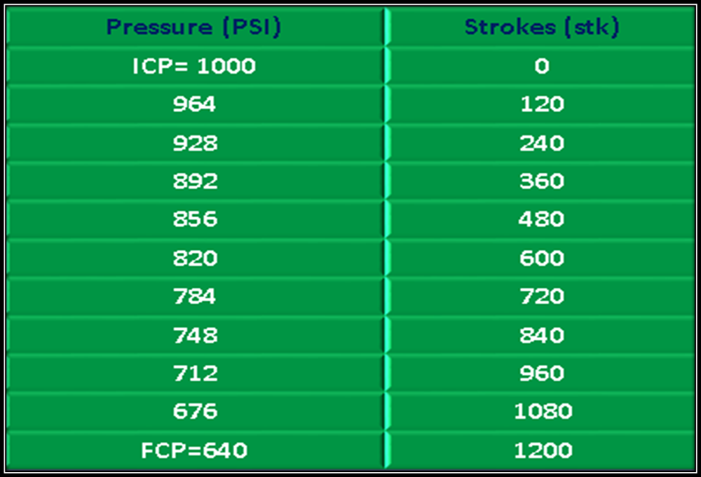
If the 1200 strokes are divided by 10, this to make the table of the engineer's method, we have 1200 strokes divided by 10, which gives us a total of 120 strokes, so we can understand the pressure drop by multiplying the 120 strokes x 0.30 psi / strokes, which would give us a pressure drop of 36 psi for every 120 strokes.

Having obtained all these results, we make the following table:

Practically the mathematics explained in this publication is to be used in the control of the well using the engineer's method technique, this considering that this is the most recommendable method as long as we have the resources needed in location.

Conclusion and contributions to engineering

The math used in well control is quite basic, however the complexity of using and applying many of the equations used in well control will depend on the field engineer's calculation skills.

As it has been shown, much of the data used to substitute for many of the equations used will depend on the ability of the driller to take certain readings at well completion, such as both drill pipe and casing completion readings.

The contribution that this publication has from the engineering point of view is that the accuracy of the calculations made at the time of well control by the engineer's method are very important, since with these calculations a drilling fluid with a new density will be prepared, in case the calculations are wrong, there is a danger that an influx of unwanted fluids such as oil and natural gas will re-enter the well and may cause a blowout at the surface, bringing human and material losses.

Note: All the images shown in this post are my own and were created using Microsoft PowerPoint design tools

References consulted and recommended

Well-control. slideshare